Radiative Transfer
Radiative transfer (RT) is the bookkeeping that turns a stellar atmosphere
into a spectrum: how the light produced and absorbed at every depth
combines into the photons that finally escape from the surface. pykurucz
solves the 1-D plane-parallel transfer equation with a JOSH-style scheme,
the same algorithm used by Fortran SYNTHE, ported line-for-line into
synthe_py/engine/radiative.py and atlas_py/physics/josh.py.
This page builds the picture in three layers: the intuition for what the equation means, the derivation of the discrete system pykurucz actually solves, and the implementation in the Python source.
Intuition
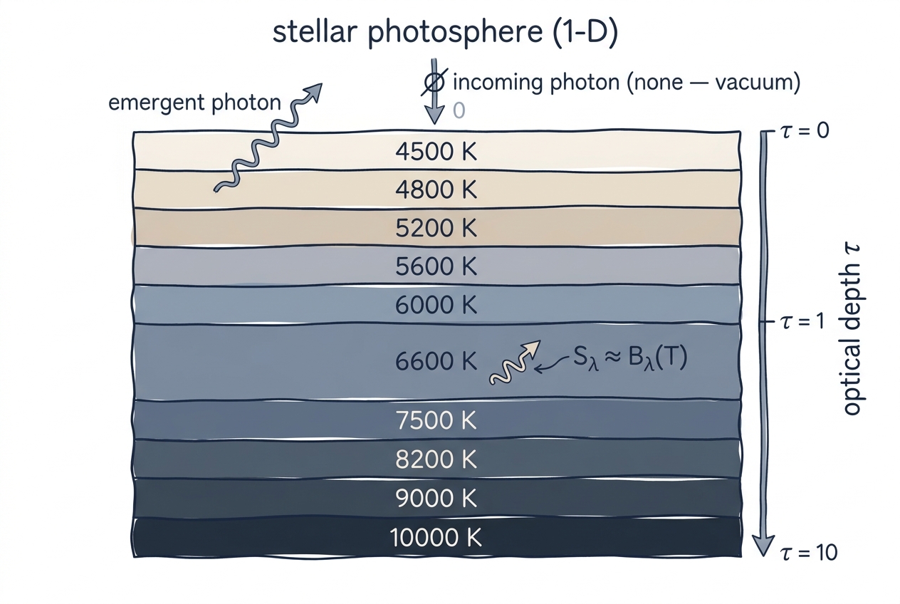
A 1-D plane-parallel photosphere as a stack of layers, each emitting roughly like a blackbody at its local temperature. Photons born deep travel up through the column, being absorbed and scattered along the way; what reaches \(\tau = 0\) is the spectrum we observe.
Imagine a single column through the photosphere. At each depth the gas emits some photons (thermal radiation) and absorbs/scatters some of the photons that pass through (opacity). RT asks: given the temperature structure \(T(\tau)\) and the opacity sources, what is the emergent intensity at the top of the atmosphere?
For a stationary 1-D atmosphere in LTE, the answer reduces to balancing two competing processes at every layer:
- Emission: each parcel radiates roughly like a blackbody at its local temperature, \(S_\lambda \approx B_\lambda(T)\).
- Absorption: photons travelling through the parcel are attenuated by \(e^{-\Delta\tau}\) across an optical-depth element \(\Delta\tau\).
The trick is that "the radiation field at depth \(\tau\)" depends on the emission everywhere else in the column. So even though there is no time-dependence, the equation is non-local — and that's what JOSH solves.
Plane-parallel approximation
The plane-parallel assumption is excellent for dwarfs and subgiants but breaks down for evolved giants with extended atmospheres (\(\log g \lesssim 1\)). pykurucz, like ATLAS12, is strictly 1-D. For spherical or 3-D geometries, ingest an external atmosphere via Existing Atmosphere.
Derivation
The transfer equation
For specific intensity \(I_\lambda(\tau, \mu)\) at angle \(\mu = \cos\theta\) to the surface normal:
where \(\tau_\lambda\) is the monochromatic optical depth measured inward and \(S_\lambda\) is the source function. In LTE with no scattering, \(S_\lambda = B_\lambda(T)\).
The emergent flux is the angle-averaged outgoing intensity:
Moment form and the Eddington closure
Direct angle integration is expensive. JOSH instead solves the second-moment form of the transfer equation. Define the moments of the radiation field:
Taking \(\int d\mu\) and \(\int \mu\, d\mu\) of the transfer equation yields the coupled pair
To close this system we need a relation between \(K\) and \(J\). Deep in the atmosphere the radiation is nearly isotropic and \(K \to J/3\); this Eddington closure is exact in the diffusion limit. Combining the two moment equations with \(K = J/3\) gives a single second-order ODE for \(J\):
That is what JOSH discretises and solves.
Surface boundary condition: \(J = \tfrac{3}{2}H\) at \(\tau = 0\)
At the top of the atmosphere there is no incoming radiation (\(I_\lambda(\tau=0, \mu<0) = 0\)). For a hemispherically isotropic outward intensity ("two-stream" / Eddington at the boundary), the moments satisfy
which serves as the upper boundary condition on the second-order ODE. At the bottom of the grid (\(\tau \to \tau_{\max}\)) the diffusion approximation gives \(H = (1/3) \, dB/d\tau\).
Parabolic differencing → tridiagonal system
JOSH discretises \(J(\tau)\) on the 80-layer atlas grid. Using a parabolic fit through three consecutive depth points (\(\tau_{i-1}, \tau_i, \tau_{i+1}\)) and substituting into the second-derivative term yields a linear equation that only couples three neighbouring layers:
Stacking these for \(i = 1, \dots, N_\tau\) (with the boundary conditions above plugged into rows 1 and \(N_\tau\)) gives a tridiagonal matrix. Tridiagonal systems are solved in \(\mathcal{O}(N_\tau)\) by the Thomas algorithm — a one-pass forward elimination followed by a back substitution — much cheaper than the \(\mathcal{O}(N_\tau^3)\) cost of a generic Gaussian elimination.
Once \(J\) is known, the flux follows from
evaluated as a finite difference of \(J\) on the depth grid.
Scattering: \(\Lambda\) iteration
When scattering matters (Thomson scattering in the UV, electron scattering in hot stars), the source function depends on \(J\) itself:
JOSH handles this with simple \(\Lambda\) iteration:
- Start with \(S^{(0)} = B_\lambda\) (pure absorption).
- Solve the tridiagonal for \(J^{(n)}\).
- Update \(S^{(n+1)}\) using the formula above.
- Stop when \(|S^{(n+1)} - S^{(n)}|/S^{(n)} < \varepsilon\).
In synthe_py, the tolerance is set by --scat-tol (default 1e-3)
and the maximum number of iterations by --scat-iterations (default 8).
\(\Lambda\) iteration vs. ALI
Plain \(\Lambda\) iteration converges slowly when scattering is optically thick, because each iteration only propagates information by one mean free path. Accelerated \(\Lambda\) Iteration (ALI) or Ng acceleration would converge in many fewer iterations and could be added to a future version. For typical optical/NIR synthesis the 8-iteration default is fine; you only see the limitation in deep UV resonance lines.
How abundance changes propagate
The JOSH solver itself is abundance-agnostic: it integrates the moment ODE for \(J\) given a total opacity \(\kappa_{\rm tot}\) and a source function \(S_\lambda\) supplied by the caller. Abundance information enters one layer up — through KAPP/COOLOP (continuum) and the line opacity loop, both of which read the per-element abundance vector described in Opacity → How abundance changes propagate. RT just sees the result.
This separation is what lets the same JOSH code handle a solar spectrum and a CEMP-s spectrum without modification: the sole difference between the two runs is the \(\kappa_{\rm tot}\) and \(S_\lambda\) vectors that the upstream opacity/EOS layer hands to JOSH.
Implementation
The Python implementation lives in two places that share the same JOSH core:
| File | Role |
|---|---|
synthe_py/engine/radiative.py |
Per-wavelength solver called by the synthesis loop |
atlas_py/physics/josh.py |
Identical algorithm called inside atlas_py iteration |
For each frequency point both files perform the same six steps, in order:
- Build opacity / source vectors from the atmosphere —
ACONT,ALINE,SIGMAC,SIGMAL,SLINE,SCONTarrays at every depth. - Total opacity \(\kappa_{\rm tot} = \kappa_{\rm cont} + \kappa_{\rm line} + \sigma_{\rm scat}\).
- Assemble the tridiagonal coefficients \((a_i, b_i, c_i)\) from the parabolic differencing of the moment ODE.
- Thomas algorithm to solve for \(J\).
- Finite-difference \(H\) from \(J\) and the boundary conditions.
- Surface BC \(J = \tfrac{3}{2}H\) at \(\tau = 0\) enforced exactly.
If scattering is enabled, steps 3–6 are wrapped in the \(\Lambda\) loop.
Fortran provenance & safety clamps
Each step of the Python implementation traces back to a labelled
block in Fortran JOSH. The original Fortran clamps negative
HNU values to a small positive floor; the Python translation
reproduces this clamp exactly to avoid unphysical flux dips in
strong scattering lines.
Performance
JOSH is called once per wavelength point. For a full 300–1800 nm synthesis at \(R = 300{,}000\) this is \(\sim\)45 000 calls. Each call solves an \(N_\tau \times N_\tau\) tridiagonal (\(N_\tau = 80\), so the solve itself is cheap), but cumulative cost matters:
- Numba JIT: the inner solver is JIT-compiled, dropping per-call overhead to \(\sim\)10–100 µs.
- Wavelength parallelism: the 45 000 calls are independent and are distributed across CPU cores by the synthesis driver.
Next Steps
- Learn about the opacity sources that fill the \(\kappa_{\rm tot}\) vector.
- Read line broadening to see how individual lines contribute to \(\kappa_\lambda\).
- See the synthe_py architecture for how the JOSH solver is plugged into the parallel synthesis loop.