Opacity
Opacity tells you how strongly the gas absorbs or scatters light at a given wavelength. It is the single quantity that links the atmosphere (\(T\), \(P\), abundances) to the spectrum, and it is the most expensive piece of the synthesis to compute correctly. pykurucz follows the Fortran convention of splitting it into continuous opacity (a smooth background from atomic ionisation, scattering, and molecular continua) and line opacity (the discrete absorption profiles of \(\sim\)1.3 million atomic transitions plus several million molecular ones).
Intuition
Continuous opacity sets the floor of the spectrum — the level at which you would see flux if there were no spectral lines. It is a broad, mostly-monotonic function of wavelength that depends on the local temperature and ionisation balance.
Line opacity adds the dips on top of that floor: every absorbing transition steals photons over a narrow wavelength interval set by its broadening profile. The line depth at a given wavelength depends on the ratio of line opacity to continuous opacity at that wavelength, which is why "the same line" looks different in a hot star versus a cool star — the continuous opacity background is different.
In the optical and near-infrared spectrum of a Sun-like star, H⁻ bound-free dominates the continuum (about 80 % of \(\kappa_{\rm cont}\) at 500 nm in the photosphere), and metal lines dominate the line opacity. Both numbers shift dramatically as you move to hot stars (Thomson scattering takes over) or cool stars (molecular bands swamp the metal lines).
Continuous Opacity Sources
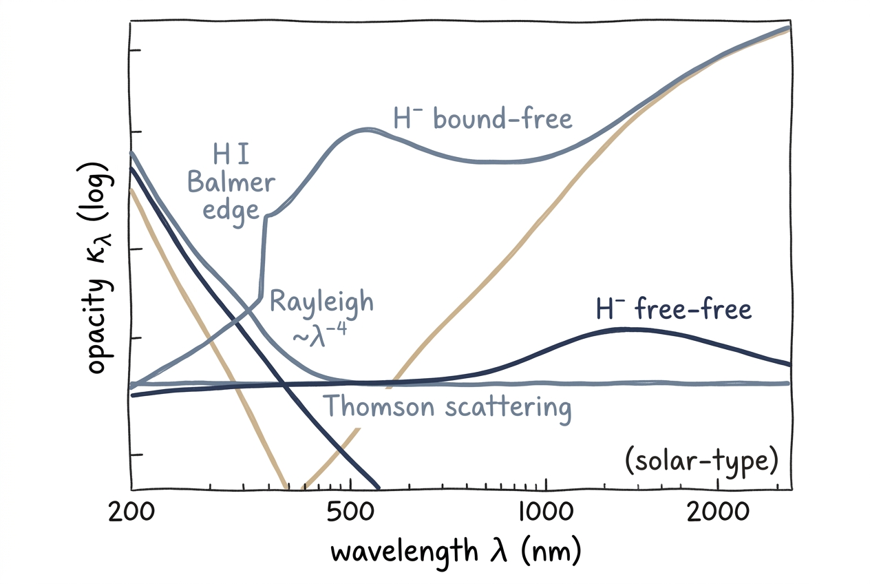
Schematic continuum opacity (log scale) vs. wavelength for a Sun-like photosphere. H⁻ bound-free dominates the optical, Rayleigh scattering rises blueward as \(\lambda^{-4}\), the Balmer edge punches the H I bound-free step at ~365 nm (vacuum), Thomson scattering is flat, and H⁻ free-free contributes broadly in the infrared. Real opacity is a sum of these (and many more).
atlas_py and synthe_py evaluate the continuum via the KAPP
subroutine (and its cool-star extension COOLOP). The contributing
processes are:
H⁻ bound-free and free-free
The negative hydrogen ion has a weakly bound state (binding energy 0.754 eV) and a large photoionisation cross-section that peaks in the optical. In solar-type stars it provides roughly 80 % of the continuous opacity at 500 nm. Bound-free cross-sections are interpolated from Mihalas-style pre-tabulated tables; free-free is computed from the Saha-populated H⁻ number density.
H I bound-free
Photoionisation from hydrogen excited states (\(n=2, 3, \ldots\)) is the dominant continuum source in the near UV, especially the Balmer (\(n=2 \to\) continuum, \(\lambda < 364.6\) nm) and Paschen edges. pykurucz follows the Karzas–Latter formulation with Gaunt factors lifted directly from the Fortran tables.
Helium
He I and He II photoionisation edges sit at their respective threshold wavelengths. He II becomes important in hot stars (\(T_{\rm eff} \gtrsim 20{,}000\) K) and Wolf–Rayet-like atmospheres.
Metal photoionisation
Photoionisation from low-lying excited states of Fe I, Mg I, Si I, and
many other metals contributes a continuous "blanket" through the UV and
blue. Cross-sections are interpolated from lines/continua.dat, which
collates the Fortran ATLAS bound-free tables.
Rayleigh scattering
Elastic scattering by neutral H, He, and H₂ rises steeply as \(\lambda^{-4}\) and dominates the continuum blueward of \(\sim\)400 nm in cool dwarfs.
Thomson scattering
Frequency-independent electron scattering, dominant in hot ionised atmospheres (O / early B stars).
Cool-star molecular continuum (COOLOP)
For \(T_{\rm eff} \lesssim 4500\) K, molecular dissociation/formation produces additional continuous opacity:
- CH and OH collisional contributions
- H₂–H₂ and H₂–He collision-induced absorption (CIA)
These are switched on automatically when MOLECULES ON is set (the
default).
Two opacity grids: atmosphere vs. synthesis
pykurucz uses two different frequency grids for opacity, matching ATLAS12 and SYNTHE conventions:
| Grid | Size | Used by | Why this size |
|---|---|---|---|
| Atmosphere grid | ~3000 frequency points spanning 9.1 nm – 10 µm | atlas_py during convergence iteration |
Coarse enough to be cheap to recompute every iteration; dense enough to integrate the radiative flux to good accuracy |
| Synthesis grid | \(\lambda/\Delta\lambda\) at the requested --resolution (~45 000 points for 300–1800 nm at \(R=300{,}000\)) |
synthe_py during line-by-line synthesis |
Spectral output grid; resolves every line profile |
When you change --wl-start, --wl-end, or --resolution, only the
synthesis grid changes. The 3000-point atmosphere grid is fixed by
the underlying ATLAS tables and is independent of the user request.
Line Opacity
Atomic lines
The Kurucz GFALL catalog lines/gfallvac.latest contains approximately
1.3 million atomic transitions. For each line, pykurucz computes:
- Line-centre opacity — proportional to \(f\)-value \(\times\) lower-level population from Saha–Boltzmann.
- Voigt profile — convolution of the Doppler (Gaussian, thermal + microturbulent) and damping (Lorentzian, natural + Stark + van der Waals) components.
- Wing accumulation — opacity is added to the synthesis grid out to
the far wings, truncated where it falls below
CUTOFF * CONTINUUM.
See line broadening for the Voigt machinery.
Molecular lines
Molecular opacity is on by default when data/molecules/ is populated.
The supported sources are:
- TiO — Schwenke binary line list (
schwenke.bin) - H₂O — Partridge–Schwenke binary line list (
h2ofastfix.bin) - Kurucz ASCII catalogues — CH, OH, CO, CN, C₂, MgH, SiH, FeH, and about 50 species in total
Molecular lines use the same Voigt machinery as atoms; their populations come from the molecular equilibrium solver (see Molecular Equilibrium).
Turning off molecules
--no-molecular-lines disables every molecular contribution; use
--no-tio or --no-h2o to drop one specific binary while keeping
the ASCII catalogues.
Opacity Cutoff
To stop every line from contributing to the entire spectrum, SYNTHE truncates each profile where it would only matter at the sub-millicontinuum level:
The default CUTOFF = 1e-3 matches Fortran SYNTHE. Lowering it (e.g.
--cutoff 1e-4) includes more weak lines and far-wing opacity at
roughly linear cost in run time. Raising it speeds up synthesis at the
expense of fidelity in dense line forests.
How abundance changes propagate
Both the continuum (KAPP) and the line-opacity (LINES) paths consume
the same per-element abundance vector that lives on the atmosphere
object: atlas_py.physics.kapp takes a 99-element xabund array as
input, and synthe_py.physics.mol_populations calls
_build_xabund_from_atm(atm) to reconstruct the same array on the
synthesis side. So when you change a --mh/--am knob or set a
per-element override with --abund, the entire opacity stack
recalculates against the new pattern with no special-case branches:
- Continuum: H⁻ population scales with the new electron donor
abundances; metal photoionisation scales with the per-species
number density (
xabund[Z]); Rayleigh and Thomson pieces scale with the resulting H and free-electron densities. - Lines: each transition's line-centre opacity is proportional to
the lower-level population, which is in turn proportional to the
element's
xabundafter Saha–Boltzmann ionisation balance. - Molecules: see
Molecular Equilibrium — the equilibrium
solver receives the same
xabundand recomputes partial pressures consistently.
This is what makes the ATLAS12-style direct opacity sampling worthwhile: there is no abundance-pattern-dependent re-tabulation of opacity tables to redo.
Implementation
| Subroutine | Where | Role |
|---|---|---|
KAPP (atlas_py/physics/kapp.py, synthe_py/engine/opacity.py) |
both | Continuous opacity (H⁻, H I, He, metal b-f, Rayleigh, Thomson) |
COOLOP (atlas_py/physics/coolop.py) |
atlas only | Cool-star molecular continuum + CIA |
LINES / wing accumulation (synthe_py/physics/lines.py) |
synthe only | Atomic and molecular line opacity into the synthesis grid |
The atmosphere code calls KAPP every iteration on the 3000-point grid. The synthesis code calls KAPP once on the high-resolution synthesis grid and then folds the line opacities on top.
Next Steps
- Read line broadening for the Voigt-profile details that govern the per-line shape.
- Explore molecular equilibrium for how molecular populations feed the line-opacity machinery.
- See hydrogen & helium for the special-case treatment of the most abundant elements.