Hydrogen & Helium

Hydrogen and helium dominate the mass and the opacity budget of almost every stellar atmosphere. Their lines need special machinery: hydrogen because the linear Stark effect makes its profiles fundamentally non-Voigt, helium because its complex term structure forces the use of tabulated profiles instead of first-principles calculations.

Intuition

For most metal lines, the line shape is set by independent broadening mechanisms (Doppler, natural, van der Waals, quadratic Stark) that combine into a Voigt profile (see line broadening).

Hydrogen breaks that picture in two places:

1. The linear Stark effect. Because the unperturbed energy levels of hydrogen are degenerate in \(\ell\), an electric microfield causes the levels to split linearly in field strength. The ensemble distribution of microfields produced by the surrounding plasma — the Holtsmark distribution — is much broader than a Lorentzian, and the ensemble-averaged line shape has long, slowly-falling wings that no Voigt fit can reproduce.
2. Strong continuum coupling. H⁻ is the dominant continuum opacity for solar-type stars in the optical, and any error in the neutral-H number density propagates straight into the predicted continuum level.

Helium is its own kind of mess: dozens of overlapping lines from singlet and triplet systems, multiple metastable levels, and electron collisions strong enough that the broadening cannot be computed from first principles. The solution is to tabulate the line shapes from quantum calculations and interpolate at synthesis time.

Hydrogen lines

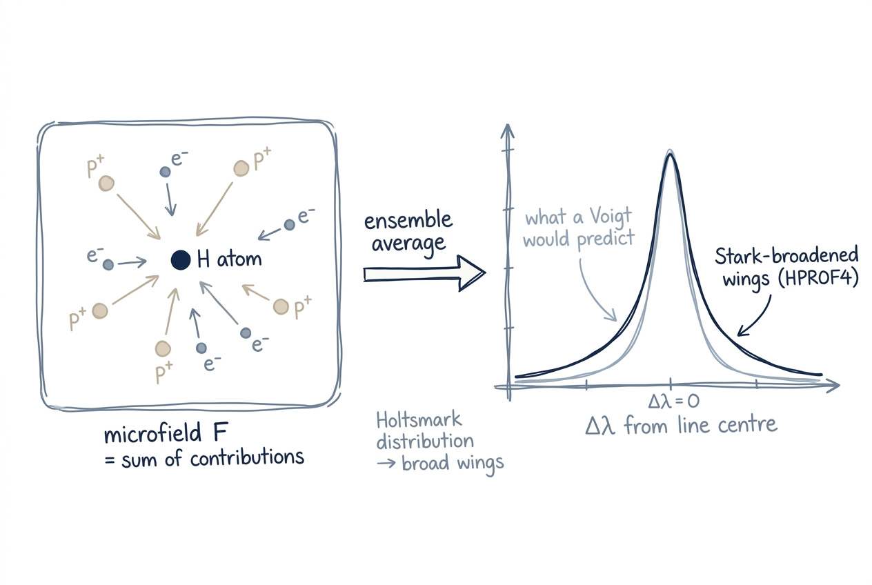
Neighbouring electrons and ions each contribute an electric field at the absorbing H atom; the ensemble of those microfields follows the Holtsmark distribution, much broader than a Lorentzian. The resulting line profile (right) has wings that no Voigt fit can reproduce — pykurucz uses HPROF4 tables instead.

Stark broadening tables (HPROF4)

For each Balmer / Lyman / Paschen / etc. line, pykurucz reads the HPROF4 profile tables — the same precomputed Stark profiles used by Fortran SYNTHE — and interpolates them in (electron density, temperature, \(\Delta\lambda\)) space to produce the local line opacity at every depth. The data carry the integrated Holtsmark microfield and the hydrogenic wave-function overlap, so the resulting profile is correct in the wings (where pure Voigt would be wrong) and in the core (where the static-microfield approximation holds).

The function compute_hydrogen_wings() in synthe_py/physics/hydrogen_wings.py interpolates the HPROF4 tables to fill the synthesis-grid arrays AHLINE (absorption) and SHLINE (source function) for every depth and every wavelength near a hydrogen line.

Hydrogen continuum

Hydrogen also dominates the continuum:

• H⁻ bound–free — peaks in the optical; provides about 80 % of \(\kappa_{\rm cont}\) at 500 nm in the solar photosphere.
• H⁻ free–free — important in the IR, scaling with electron density.
• H I bound–free from \(n=2, 3, …\) — Balmer / Paschen / Brackett edges. The Balmer edge sits near 364.6 nm (vacuum), the Paschen edge near 820.4 nm (vacuum). These thresholds are extremely sharp in the spectrum.
• Thomson scattering off the free electrons released by H ionisation, frequency-independent.

These are evaluated in the KAPP / COOLOP path alongside the metal and helium continua (see opacity).

Why H⁻ dominates

The negative hydrogen ion has a weakly bound state (binding energy 0.754 eV) and a large photoionisation cross-section that peaks in the optical. In the Sun, H⁻ provides ~80 % of the continuous opacity at 500 nm. Inaccurate H⁻ opacity throws off the predicted continuum level and therefore the depths of all the lines on top of it.

Helium lines

Tabulated profiles (he1tables.dat)

For He I, pykurucz loads tabulated line broadening profiles from lines/he1tables.dat (and the corresponding pre-extracted synthe_py/data/he1_tables.npz). The tables cover:

• He I lines broadened by electrons (Stark) and neutrals (van der Waals), with parameters drawn from Griem and from Dimitrijević–Konjević calculations.
• The strongest transitions in the visible / NIR; weaker He I lines fall back to the generic Voigt path.

The runtime helper helium_profiles.py interpolates these tables and matches the Fortran HE1LINE subroutine bit-for-bit.

Helium Voigt batch kernel

He I lines without explicit tabulated profiles fall back to the standard Voigt with catalog damping constants. Because He I lines are densely packed in the UV (every \(n \to n'\) transition with all the fine-structure components), pykurucz uses a dedicated Numba batch kernel (_compute_helium_voigt_batch) to evaluate many of them in a single pass.

How abundance changes propagate

H and He are special: He is fixed at the constant HE_ABUNDANCE = 0.078370 (mass fraction) — it is not a user knob, matching the standard ATLAS convention. H is computed by mass conservation: compute_h(mh, am, individual) in pykurucz.py sets \(X_{\rm H} = 1 - X_{\rm He} - \sum_{Z \ge 3} 10^{A_Z}\). So when you change --mh, --am, or any per-element --abund, \(X_{\rm H}\) adjusts slightly to keep the total fraction unity. The shift is small in the typical regime (metals are trace) but matters at very high metallicity.

The HPROF4 Stark tables for H lines and the he1tables.dat profiles for He I lines are abundance-independent quantum-mechanical tables — they capture how a hydrogen or helium atom responds to electric microfields, not how many of them are present. The actual line widths used at synthesis time still depend on abundance, because they fold the table with the local electron density \(N_e\) (set by Saha–Boltzmann ionisation, which depends on every donor in the gas). So a metal-poor halo dwarf and a solar dwarf use the same HPROF4 tables but produce noticeably different Balmer wings, because the electron-donor budget is different.

The H⁻ and metal-photoionisation continuum pieces are abundance-driven through the same Saha–Boltzmann path; see Opacity → How abundance changes propagate.

Why this matters

Skipping any of the hydrogen / helium machinery produces visible errors:

Skipped	Visible failure mode
HPROF4 hydrogen Stark tables	Balmer lines too narrow (no proper wings) in A and early-F stars
He I tabulated profiles	UV He I region wrong in B stars
H⁻ continuum	Continuum level off → all line depths off in solar-type stars
H I bound-free edges	Sharp continuum jumps at the Balmer/Paschen/Brackett edges missing

Implementation

File	Role
synthe_py/physics/hydrogen_wings.py	HPROF4 interpolator (compute_hydrogen_wings)
synthe_py/physics/helium_profiles.py	He I tabulated-profile interpolator
synthe_py/physics/voigt_jit.py	_compute_helium_voigt_batch for He I lines without tables
atlas_py/physics/kapcont.py (and synthe_py/engine/opacity.py)	H⁻ b-f, H⁻ f-f, H I b-f, Thomson

Next Steps

• See line broadening for the generic Voigt machinery used by all non-H/He lines (and by He I lines without dedicated tables).
• See opacity for the full picture of how H/He continuum interleaves with metal and molecular lines.
• See radiative transfer to follow what happens once the opacity grid is built.