Line Broadening

Spectral lines are never infinitely narrow. Three independent mechanisms spread the absorption (and emission) over a finite wavelength interval: the natural linewidth set by quantum lifetimes, Doppler broadening from the thermal/turbulent motion of absorbers, and pressure broadening from collisions. pykurucz combines them into a single Voigt profile for every atomic and molecular transition.

Intuition

Two qualitative shapes matter:

• Doppler core: a Gaussian, narrow and tall, set by the root-mean-square radial velocity of atoms in the gas (thermal + microturbulent).
• Damping wings: a Lorentzian, wide and shallow, set by the sum of natural, Stark, and van der Waals damping constants.

Because the two are independent, the actual line shape is the convolution of a Gaussian and a Lorentzian — the Voigt function. At low pressure the core dominates and the line looks Gaussian; at high pressure the wings dominate and the line looks Lorentzian. Most metal lines in solar-type stars sit in the regime where both contribute.

A useful single number is the dimensionless damping parameter

\[ a = \frac{\gamma}{4\pi\,\Delta\nu_D}, \]

the ratio of the Lorentzian half-width to the Gaussian Doppler width. \(a \ll 1\) means the line is essentially Gaussian; \(a \sim 1\) means the wings are visible; \(a \gg 1\) rarely happens in stellar photospheres except for the strongest resonance lines.

Derivation

Natural broadening

The radiative lifetime of an excited state sets a fundamental width via the energy–time uncertainty relation:

\[ \gamma_{\rm rad} = \frac{4\pi e^2}{m_e c}\sum_j f_{ij} \;=\; 0.2223 \times 10^8\,\text{s}^{-1} \times \sum_j f_{ij} . \]

The GFALL catalog supplies \(\gamma_{\rm rad}\) directly per transition (in \(\log_{10}\) form). It is usually the smallest of the three damping contributions except for strong resonance and forbidden lines.

Stark broadening

Charged-particle perturbations dominate for hydrogen (linear Stark) and for any high-\(n\) transition (quadratic Stark). For non-hydrogen lines, GFALL supplies a coefficient that is multiplied by the local electron density:

\[ \gamma_{\rm Stark} = \gamma_{\rm Stark}^{(\text{cat})} \times N_e . \]

Hydrogen Stark broadening

Hydrogen Balmer and Lyman lines are not handled by the generic Voigt path — they need the dedicated HPROF4 tables (see Hydrogen & Helium). The Voigt code below is used for everything else.

van der Waals broadening

Collisions with neutral hydrogen (and to a lesser extent He) are the dominant pressure mechanism for most metal lines in cool and solar-type stars:

\[ \gamma_{\rm vdW} = \gamma_{\rm vdW}^{(\text{cat})} \times N_{\rm H} \times \left(\frac{T}{10^4\,\text{K}}\right)^{0.3} , \]

where \(N_{\rm H}\) is the neutral hydrogen number density. The temperature exponent 0.3 is the classical Unsöld approximation; a fraction of GFALL lines carry more accurate exponents from quantum calculations (encoded in the LOG GAMMA column of the catalog).

Doppler width

The thermal velocity includes both thermal and microturbulent broadening:

\[ v_D = \sqrt{\frac{2 k_B T}{m_a} + v_{\rm turb}^2} , \]

where \(m_a\) is the atomic mass of the absorber. The Doppler width in wavelength is then \(\Delta\lambda_D = \lambda_0 v_D / c\).

Voigt profile

The Voigt function is the convolution of a Gaussian (Doppler) and a Lorentzian (damping):

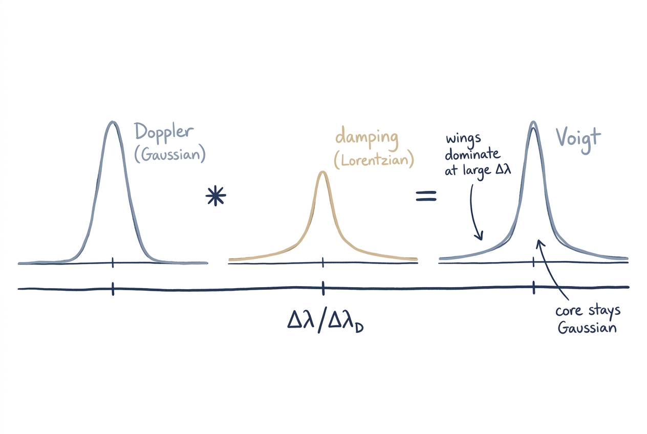
The narrow Gaussian (Doppler) core convolved with the slowly-decaying Lorentzian (damping) wings produces the Voigt profile on the right. The core stays Gaussian; the wings are dominated by the Lorentzian.

\[ H(a, x) = \frac{a}{\pi} \int_{-\infty}^{\infty} \frac{e^{-y^2}}{(x - y)^2 + a^2} \, dy , \]

with

• \(x = \Delta\lambda / \Delta\lambda_D\) — displacement from line centre in Doppler units,
• \(a\) — the damping parameter defined above.

Numerically the Voigt function is the real part of the Faddeeva function, \(H(a, x) = \mathrm{Re}\,w(x + ia)\), where \(w(z)\) is computed by scipy.special.wofz. This is the high-accuracy reference path.

Why a fast lookup table for \(a < 0.2\)

The Faddeeva function is accurate everywhere but expensive — each call costs hundreds of nanoseconds. In a synthesis loop we evaluate the profile at ~20 points per line for ~1 million lines, so the cost adds up.

For the vast majority of metal lines in cool stars, the damping parameter satisfies \(a < 0.2\). In that regime, the Voigt function can be expanded as

\[ H(a, x) \;\approx\; H_0(x) + a\, H_1(x) + \mathcal{O}(a^2) , \]

i.e. a linear interpolation in \(a\) between two pre-computed profiles. pykurucz tabulates \(H_0\) and \(H_1\) on a fixed \(x\)-grid matching Fortran SYNTHE, and at synthesis time looks them up in \(\mathcal{O}(1)\).

Why the cutoff at \(a = 0.2\)? At that value the \(\mathcal{O}(a^2)\) correction term contributes a few × 10⁻⁴ relative error in the profile core — about the same level as the SYNTHE opacity-cutoff threshold. Above \(a = 0.2\) the linear expansion would introduce visible deviations, so the code falls back to the full Faddeeva path. The value is identical to the threshold used by the Fortran code, ensuring numerical parity.

How abundance changes propagate

The Voigt shape (Gaussian × Lorentzian convolution) is intrinsic to each transition's atomic data and does not depend on abundance. What does depend on abundance is what the shape gets multiplied by:

• Line-centre opacity \(\propto\) lower-level population, which is \(f\)-value \(\times\, N_{\rm species}\), which scales linearly with the element's abundance. Shifting --abund Fe:-1.0 makes every Fe line ~10× shallower (in the optically-thin regime); going to Fe:+0.5 makes them ~3× deeper.
• Damping parameter \(a\) = (Lorentzian half-width) / (Doppler width). The Lorentzian half-width sums natural (\(\gamma_{\rm rad}\), fixed by the transition itself), Stark (\(\gamma_{\rm Stark} \times N_e\)), and van der Waals (\(\gamma_{\rm vdW} \times N_{\rm H} \times (T/10^4)^{0.3}\)) contributions. Both \(N_e\) and \(N_{\rm H}\) depend on the abundance pattern through Saha–Boltzmann ionisation balance and the \(H = 1 - He - \sum_{\rm metals}\) closure, so the wings shift slightly even for non-Fe lines when you change --mh or any per-element offset.

That is why pushing carbon up by a dex (--abund C:+1.0) does not just deepen carbon lines — it also nudges every neighbouring metal line's wings via the changed electron-donor balance and the C-bearing molecular blanketing in the upstream atmosphere.

Wing accumulation

Once the per-line profile shape is known, the opacity is added to the synthesis wavelength grid. The accumulation strategy mirrors Fortran SYNTHE labels 320–350:

1. Near wing — evaluate the profile at N10DOP = int(10 * DOPPLE * RESOLU) points centred on the line.
2. Cutoff check — once the local profile drops below KAPMIN = CUTOFF * CONTINUUM, stop the near-wing evaluation early.
3. Far wing — if the near wing finished before hitting cutoff, extrapolate as \(X / n^2\) (Lorentzian asymptote) out to MAXSTEP points.
4. Accumulate — add red and blue wing contributions to the global opacity array; no per-step cutoff once we are past step 1.

Implementation

File	Role
synthe_py/physics/voigt.py	Reference Voigt evaluation via scipy.special.wofz
synthe_py/physics/voigt_jit.py	Numba-JIT'd lookup-table path (H0TAB, H1TAB) for \(a < 0.2\)
synthe_py/physics/lines.py	Wing-accumulation loop driving the line opacity into the synthesis grid

The lookup tables H0TAB and H1TAB are pre-computed on a 200-step \(x\)-grid matching the Fortran spacing (so identical line wings are produced as Fortran SYNTHE within floating-point accuracy). The JIT kernel selects fast vs. slow path on a per-line basis.

Why the constants VSTEPS = 200, TABI = 1.5 look magic

These are the Fortran table resolution and lower-bound constants: 200 grid points per Doppler width \(\Delta\lambda_D\) across the table (more than enough to resolve the core shape with linear interpolation), and TABI = 1.5 is the lower edge of the abscissa grid in Fortran (it indexes into a table whose first element starts at \(x = -7.5\)). They are reproduced bit-for-bit so that line wings match to floating-point precision.

Next Steps

• See hydrogen & helium for the dedicated Stark-broadened H profiles and tabulated He profiles that bypass this Voigt path.
• See opacity for how line and continuous opacities combine into \(\kappa_{\rm tot}\).
• See radiative transfer to follow what JOSH does once the opacity grid is built.