High vs. Low Resolution¶

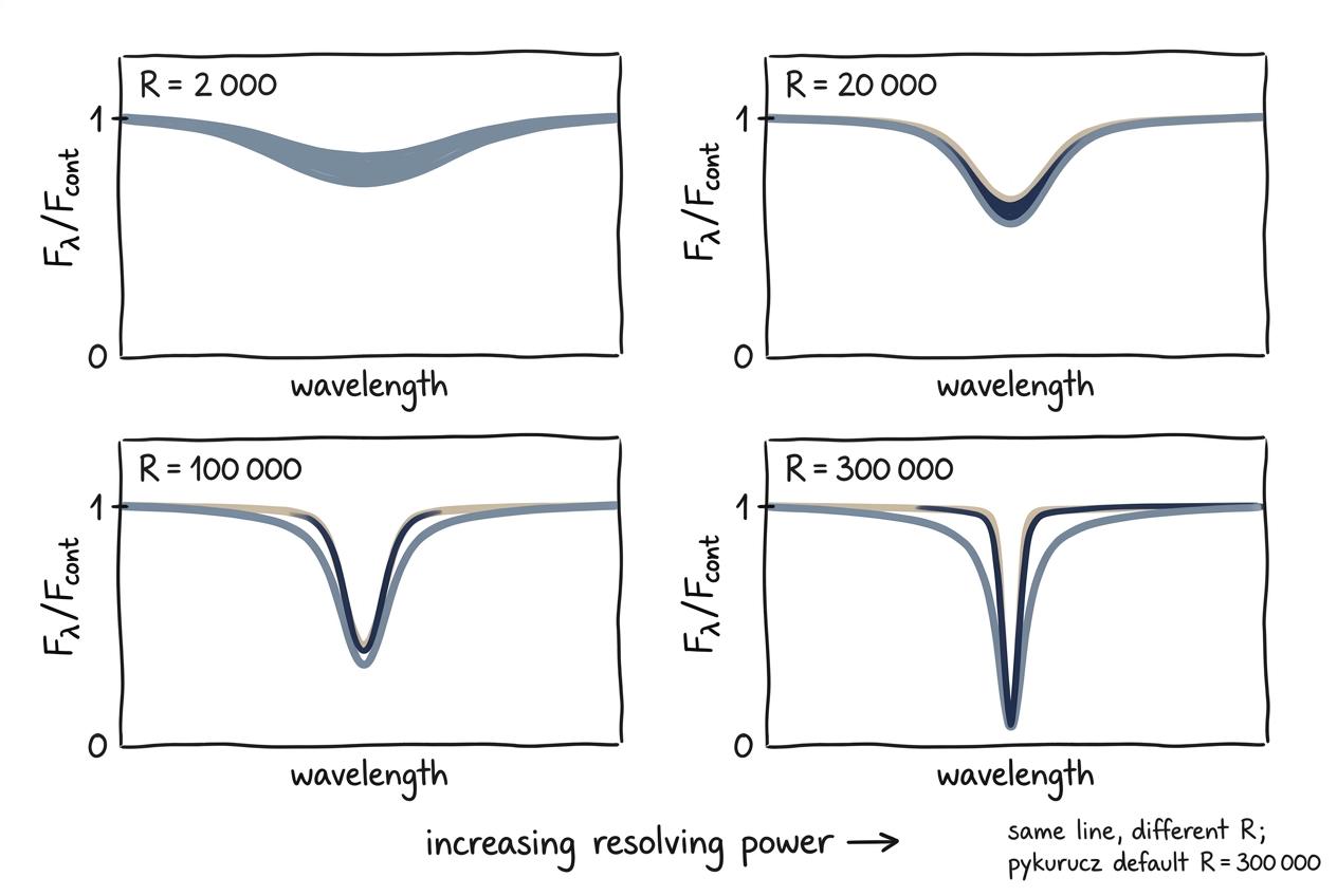
Same line at four resolving powers — The same absorption line at four resolving powers. At \(R = 2{,}000\) it is barely a saucer; by \(R = 300{,}000\) (pykurucz's default) the sharp Voigt core and extended wings are fully resolved. Match \(R\) to your instrument to keep your synthesis honest.

The choice of spectral resolution is one of the most important trade-offs in spectrum synthesis. High resolution reveals the full line profile shape and resolves blended multiplets; low resolution runs faster and is often sufficient for broad-band photometric or survey comparisons. This tutorial shows how to generate and compare spectra at three characteristic resolutions.

What You Will Learn¶

How the resolution= parameter controls the wavelength sampling
The runtime trade-off between \(R=300\,000\), \(50\,000\), and \(1\,000\)
When to synthesize at native resolution and when to convolve a high-\(R\) grid
How to overplot spectra for visual comparison

Prerequisites¶

Familiarity with the Stellar Parameters pipeline
numpy, scipy, and matplotlib installed

The Resolutions We Will Compare¶

Resolution	Context	Typical Use Case
\(R=300\,000\)	Echelle spectrograph (e.g., HARPS, ESPRESSO)	Detailed line-profile analysis, bisector studies
\(R=50\,000\)	High-resolution spectrograph (e.g., X-Shooter, MIKE)	Chemical abundance work, RV monitoring
\(R=1\,000\)	Survey photometry / low-res spectrograph (e.g., LAMOST, Gaia RVS)	Stellar parameter estimation, broad feature fitting

Resolving power definition

pykurucz uses \(R = \lambda / \Delta\lambda\) to set the uniform log-spacing of the wavelength grid. The number of points scales linearly with \(R\) and with the logarithmic wavelength span. A full 300–1800 nm synthesis at \(R=300\,000\) contains ~5.5 million pixels.

Step 1 — Run Three Resolutions¶

We use the same stellar parameters and wavelength range so that any difference is purely due to sampling. We select a 50 nm chunk around the Mg b triplet and Na D lines — a region rich with narrow metal lines.

Python scriptCLI (sequential)

from pykurucz import synthesize
from pathlib import Path

teff, logg, mh, am = 5770, 4.44, 0.0, 0.0
wl_start, wl_end = 515.0, 565.0  # Mg b + Na D region

resolutions = [300_000, 50_000, 1_000]
spec_paths = {}

for R in resolutions:
    print(f"\n=== Synthesizing at R={R:,} ===")
    spec_path = synthesize(
        teff=teff,
        logg=logg,
        mh=mh,
        am=am,
        wl_start=wl_start,
        wl_end=wl_end,
        resolution=R,
        output_dir=f"results_res_{R}",
    )
    spec_paths[R] = spec_path

for R in 300000 50000 1000; do
    python pykurucz.py \
        --teff 5770 --logg 4.44 \
        --wl-start 515 --wl-end 565 \
        --resolution $R \
        --output-dir "results_res_${R}"
done

Runtime estimate

Runtimes on an 8-core workstation for the 50 nm window above:

Resolution	synthe_py time	Total time
\(R=300\,000\)	~2–4 min	~5–8 min
\(R=50\,000\)	~20–40 s	~3–5 min
\(R=1\,000\)	< 5 s	~2–4 min

The atlas_py atmosphere iteration dominates the total time only at very low resolution; at high \(R\), synthesis is the bottleneck. For a full 300–1800 nm range, the ratio is even more extreme.

Step 2 — Load and Compare¶

All three outputs cover the same wavelength window, but the pixel counts differ dramatically:

import numpy as np

for R in [300_000, 50_000, 1_000]:
    wl, fl, ct = np.loadtxt(
        f"results_res_{R}/spec/t05770g4.44_mh+0.00_am+0.00_515_565.spec",
        unpack=True
    )
    print(f"R={R:>7,}: {len(wl):>7,} pixels,  spacing={np.mean(np.diff(wl))*1e3:.3f} pm")

The output should show something like:

R=300,000: 160,168 pixels,  spacing=0.312 pm
R= 50,000:  32,034 pixels,  spacing=1.561 pm
R=  1,000:     641 pixels,  spacing=78.023 pm

At \(R=1\,000\), the Mg b triplet (spanning ~1.6 nm) is sampled with only ~20 pixels — enough to see the blended feature as a single broad depression, but not to resolve the three components.

Step 3 — Plot the Comparison¶

The following script overplots the three resolutions and includes zoom panels for the Mg b and Na D regions.

import numpy as np
import matplotlib.pyplot as plt

def load_spec(R):
    path = f"results_res_{R}/spec/t05770g4.44_mh+0.00_am+0.00_515_565.spec"
    wl, fl, ct = np.loadtxt(path, unpack=True)
    return wl, fl / ct

fig = plt.figure(figsize=(12, 9))
gs = fig.add_gridspec(3, 1, height_ratios=[1, 1, 1])

# --- Full range ---
ax0 = fig.add_subplot(gs[0])
colors = {300_000: "C0", 50_000: "C1", 1_000: "C2"}
labels = {300_000: r"$R=300\,000$", 50_000: r"$R=50\,000$", 1_000: r"$R=1\,000$"}

for R in [300_000, 50_000, 1_000]:
    wl, norm = load_spec(R)
    ax0.plot(wl, norm, lw=0.5 if R >= 50_000 else 1.5,
             c=colors[R], alpha=0.9, label=labels[R])

ax0.set_ylabel(r"$F_\lambda / F_{\rm cont}$")
ax0.set_ylim(0, 1.1)
ax0.set_xlim(515, 565)
ax0.legend(loc="lower left")
ax0.set_title("Resolution Comparison: Solar Spectrum (515–565 nm)")

# --- Mg b zoom ---
ax1 = fig.add_subplot(gs[1])
for R in [300_000, 50_000, 1_000]:
    wl, norm = load_spec(R)
    mask = (wl >= 516.0) & (wl <= 519.0)
    ax1.plot(wl[mask], norm[mask], lw=0.5 if R >= 50_000 else 1.5,
             c=colors[R], alpha=0.9)

ax1.axvline(516.73, color="gray", ls="--", lw=0.5)
ax1.axvline(517.27, color="gray", ls="--", lw=0.5)
ax1.axvline(518.36, color="gray", ls="--", lw=0.5)
ax1.set_ylabel(r"$F_\lambda / F_{\rm cont}$")
ax1.set_ylim(0, 1.1)
ax1.set_xlim(516, 519)
ax1.set_title("Mg b Triplet Zoom")

# --- Na D zoom ---
ax2 = fig.add_subplot(gs[2])
for R in [300_000, 50_000, 1_000]:
    wl, norm = load_spec(R)
    mask = (wl >= 588.0) & (wl <= 590.5)
    ax2.plot(wl[mask], norm[mask], lw=0.5 if R >= 50_000 else 1.5,
             c=colors[R], alpha=0.9)

ax2.axvline(588.99, color="gray", ls="--", lw=0.5)
ax2.axvline(589.59, color="gray", ls="--", lw=0.5)
ax2.set_xlabel("Wavelength (nm)")
ax2.set_ylabel(r"$F_\lambda / F_{\rm cont}$")
ax2.set_ylim(0, 1.1)
ax2.set_xlim(588, 590.5)
ax2.set_title("Na D Doublet Zoom")

plt.tight_layout()
plt.savefig("resolution_comparison.png", dpi=250)

You will see:

\(R=300\,000\) (blue): Fully resolves the three Mg b components and the 0.6 nm split of the Na D doublet. Individual weak Fe I lines are visible everywhere.
\(R=50\,000\) (orange): The Mg b triplet is marginally resolved, and the Na D lines are clearly separated but with slightly shallower cores. Weak lines begin to blend.
\(R=1\,000\) (green): The entire 515–565 nm region looks like a smooth curve with a handful of broad depressions. Mg b and Na D are single unresolved features.

Native Resolution vs. Convolution¶

A common question is whether to synthesize directly at low \(R\) or to compute a high-\(R\) spectrum and convolve it with a Gaussian kernel.

Synthesize at target RSynthesize at high R and convolve

Faster: Fewer wavelength points means less line-opacity accumulation.
Self-consistent: The radiative transfer is evaluated exactly on the output grid.
Recommended when: The target \(R\) is the final science product and you do not need the high-\(R\) grid for anything else.

More flexible: One high-\(R\) synthesis can be convolved to many different resolutions.
Preserves information: You retain the option to inspect line profiles later.
Recommended when: You are building a grid for multiple instruments or doing resolution-degradation studies.

How to convolve in Python

If you choose the high-\(R\) + convolution route:

from scipy.ndimage import gaussian_filter1d
import numpy as np

# Load high-R spectrum
wl, fl, ct = np.loadtxt("results_res_300000/spec/...spec", unpack=True)
norm = fl / ct

# Target R (e.g., 50,000)
R_target = 50_000
R_native = 300_000

# Approximate Gaussian sigma in pixels
# FWHM_ratio = R_native / R_target
# sigma = FWHM_ratio / (2 * sqrt(2 * ln(2)))
sigma_pix = (R_native / R_target) / 2.355
norm_conv = gaussian_filter1d(norm, sigma=sigma_pix)

The convolution is only approximate because the line-spread function (LSF) of real spectrographs is rarely a pure Gaussian. For rigorous instrument modeling, use the spectrograph’s published LSF or a sampled kernel.

When to Use Which Resolution¶

Science Goal	Recommended \(R\)	Reason
Chemical abundance from EW	\(50\,000\)–\(100\,000\)	Lines are resolved but file size is manageable
Line bisector / profile shape	\(300\,000\)	Needs full core-to-wing sampling
Stellar parameters from broad features	\(1\,000\)–\(10\,000\)	Fast; broad bands insensitive to \(R\)
Grid generation for ML training	\(50\,000\)	Good compromise of detail and speed
Cross-correlation RV	\(300\,000\)	Maximum information content

Do not oversample

Synthesizing at \(R=300\,000\) when you only need \(R=1\,000\) wastes CPU time and disk space. The line opacity accumulation scales roughly linearly with the number of wavelength points.

Next Steps¶

Apply these resolution choices to the Solar Spectrum example to see how Balmer lines change with \(R\).
Explore the Cool Star example — molecular bandheads are much less sensitive to resolution than atomic lines.
Read the Output Files guide for tips on handling large .spec files efficiently.