Molecular Equilibrium

In cool stellar atmospheres (\(T_{\rm eff} \lesssim 4500\) K), molecules form in significant quantities and become dominant opacity sources. Accurate spectrum synthesis therefore requires solving the molecular equilibrium: the chemistry that determines the partial pressure of every molecular species at every depth in the atmosphere.

Intuition

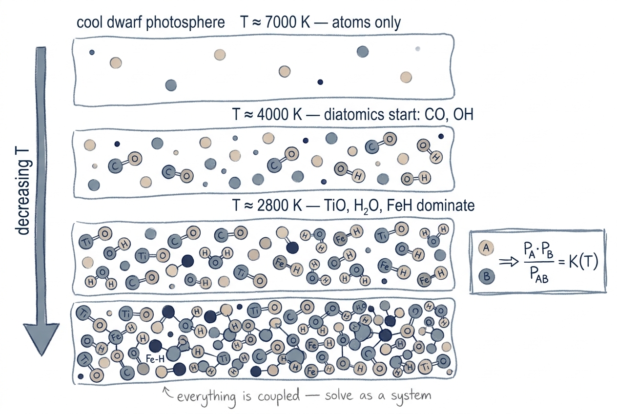
As you move down (and cool down) through a cool-dwarf photosphere, atoms first pair into simple diatomics (CO, OH at \(T \sim 4000\) K), then more complex molecules dominate (TiO, H₂O, FeH at \(T \sim 2800\) K). Every species is coupled — solving one equilibrium constant in isolation gives the wrong answer.

In hot gas, almost everything is atomic — bonds break thermally as fast as they form. As the gas cools, simple molecules (H₂, CO, OH, …) start to "freeze out": their formation energy is below \(k_B T\) and they remain bound on average. By 3000–4000 K, oxides like TiO and VO can carry several percent of the gas density and produce the characteristic broad absorption bands of M dwarfs and red giants.

The key complication is that everything is coupled: the partial pressure of TiO depends on how much atomic Ti is left, which depends on how much Ti is locked up in O-bearing molecules, which depends on how much O is left after CO formation, … Every species has to be solved simultaneously, conserving the total elemental abundance.

This is what NMOLEC does.

Derivation

Equilibrium for a single diatomic

For a generic diatomic \(AB\) with constituent atoms \(A\) and \(B\), the law of mass action gives

\[ \frac{P_A \, P_B}{P_{AB}} \;=\; K_{AB}(T) , \]

where the equilibrium constant \(K_{AB}(T)\) is set by the dissociation energy \(D_0\) and the rotational/vibrational/electronic partition functions of the three species:

\[ K_{AB}(T) \;=\; \frac{Q_A Q_B}{Q_{AB}} \, (k_B T)^{5/2} \, \frac{(2\pi m_{AB})^{3/2}}{h^3} \, e^{-D_0 / k_B T} . \]

In data/lines/molecules.dat the temperature dependence of each \(\log_{10} K(T)\) is stored as a polynomial (typically degree 4 in \(\log_{10} T\)). NMOLEC evaluates the polynomial at every depth's local \(T\) to get \(K(T)\) for each species.

The coupled system

For a real photosphere we have \(N\) atomic species and \(M\) molecular species. The unknowns are the partial pressures \(\{P_A\}\) for the atoms and \(\{P_{AB}\}\) for the molecules. The equations are:

1. Equilibrium: one equation per molecule, relating its partial pressure to those of its constituents.
2. Conservation: one equation per element, requiring the total amount of element \(X\) (free atoms + every molecule containing \(X\), weighted by stoichiometry) to equal the prescribed elemental abundance.
3. Charge neutrality / electron balance, since some molecules ionise.

That gives \(N + M\) algebraic equations in \(N + M\) unknowns. The system is non-linear because conservation couples atoms to every molecule they appear in, and molecule equilibrium couples back to atomic partial pressures.

How NMOLEC iterates

NMOLEC solves the coupled system with a fixed-point iteration on the atomic partial pressures:

1. Make an initial guess for \(\{P_A\}\) (typically: ignore molecules and take the Saha–Boltzmann atomic pressures).
2. Use the current \(\{P_A\}\) to compute every \(P_{AB}\) via mass action.
3. For each element, sum up the partial pressures (free + molecular, with stoichiometry) and compare against the target abundance.
4. Adjust \(\{P_A\}\) to reduce the residuals, and repeat from step 2.
5. Converge when every element's partial-pressure residual is below a tolerance, typically a few × 10⁻⁵ in relative terms.

The original Fortran NMOLEC uses a damped Newton-style update on \(\log P\); the Python translation reproduces the same step structure, so the same number of iterations is needed for convergence.

Species and data

atlas_py and synthe_py solve equilibrium for ~50 molecular species. The list in synthe_py/physics/mol_populations.py includes every species needed for cool dwarfs through M giants:

• Hydrides: H₂, CH, NH, OH, MgH, AlH, SiH, CaH, ScH, TiH, VH, CrH, MnH, FeH, CoH, NiH, CuH, …
• Oxides: CO, NO, O₂, SiO, MgO, AlO, CaO, ScO, TiO, VO, CrO, MnO, FeO, YO, ZrO, LaO, …
• Carbides / cyanides: C₂, CN, C₃, HCN
• Sulphides / halides: SH, SO, FH, ClH, ClO, S₂, HeH, LiH, BeH, …
• Triatomics: H₂O, CO₂

In all there are about 50 species; the exact count depends on which isotopologues are counted separately.

For each species, molecules.dat carries:

• the dissociation energy \(D_0\) in eV,
• the polynomial coefficients of \(\log_{10} K(T)\),
• isotope corrections where relevant.

Cool-star spectral signatures

The dominant molecular bands you can expect to see in cool-star spectra (approximate bandhead wavelengths, given as vacuum values consistent with pykurucz's internal convention):

Feature	Bandhead (nm)	Molecule	Stellar type
TiO γ system bandheads	~516, 544, 586, 615, 705	TiO	M dwarfs/giants
H₂O bands (NIR)	~940, 1130, 1380	H₂O	Late M, brown dwarfs
CN violet system	~388, 421	CN	Carbon stars, giants
CO first-overtone	~2300	CO	All cool stars
CH G-band	~430.5	CH	F–G dwarfs
MgH	~478	MgH	K giants

These wavelengths refer to bandheads (the sharp blue edge of a rotational-vibrational band envelope), not individual line centres. For exact line positions, consult the line lists themselves.

Why NMOLEC matters for cool stars

In a 4000 K dwarf, TiO alone can account for more than 10 % of the total opacity in the optical. Neglecting molecular equilibrium produces spectra that are systematically too blue and too shallow in molecular bands. Early pykurucz cool-star validation found a ~90 % discrepancy in the Na D doublet that traced directly to missing molecular opacity; switching MOLECULES ON resolved it.

Implementation

File	Role
atlas_py/physics/nmolec.py	NMOLEC solver invoked inside the atlas iteration
atlas_py/io/molecules.py	Parser for molecules.new / molecules.dat
synthe_py/physics/mol_populations.py	Standalone molecular-equilibrium solver used by convert_atm_to_npz

How abundance changes propagate

NMOLEC's elemental conservation constraint reads the same per-element abundance vector that the rest of the code uses (_build_xabund_from_atm in synthe_py/physics/mol_populations.py, or the xabund argument inside atlas_py/physics/nmolec.py). When you change --mh, --am, or any individual --abund Z:offset, the new abundance vector is what NMOLEC conserves against — so the partial pressures of every species are recomputed for the actual pattern, and TiO / H₂O / CO / etc. are not borrowed from a scaled-solar template. This matters in particular for CEMP-style cases where C/O > 1 flips the carbon-bearing chemistry on its head: the same code path handles it correctly with no special casing because the abundance vector is the only input that changed.

Where it runs in the pipeline:

• In Stellar Parameters, NMOLEC is invoked from inside POPSALL on every atlas_py iteration; molecular populations are written into the converged .atm and reused by synthesis.
• In Existing Atmosphere, NMOLEC is invoked once by convert_atm_to_npz.py and the populations are stored in the .npz cache; synthesis never re-solves the chemistry inside the wavelength loop.

Next Steps

• See opacity for how molecular populations turn into line opacity in the synthesis grid.
• See line broadening for the Voigt profiles applied to every molecular line.
• See the atlas_py architecture for how NMOLEC plugs into the atmosphere iteration.