Your First Spectrum
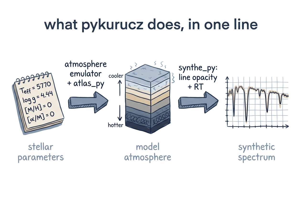
Four numbers in, one synthetic spectrum out. The atmosphere emulator + atlas_py build a self-consistent model atmosphere from your stellar parameters; synthe_py then folds line opacity and radiative transfer through that atmosphere to produce the emergent flux.
This page is a detailed walkthrough of your first end-to-end synthetic spectrum. We will generate the spectrum of a Sun-like star, inspect the intermediate outputs, and interpret the results.
Roughly what to expect
The atmosphere emulator returns its warm start essentially instantly.
The atlas_py iteration is the slow part — most of the runtime is here,
scaling with the number of iterations to convergence and how aggressively
opacity is recomputed. The synthe_py synthesis cost is set by the
wavelength range and the number of lines that fall in it; it parallelises
across CPU cores by default. A 10-nm window finishes in a small fraction
of the time of a full 300–1800 nm synthesis.
Concrete timings depend on your hardware enough that you should benchmark on your own machine rather than rely on a published number.
Step 1 — Install and Download Data
If you haven't already, follow Installation to set up the Python environment and Downloading Data to fetch the line-list binaries (~1.3 GB minimum).
Step 2 — Run the Pipeline
We will synthesize a 10 nm chunk around 500 nm for the Sun:
python pykurucz.py --teff 5770 --logg 4.44 --wl-start 500 --wl-end 510
You should see three stages in the terminal:
- Emulator warm-start — predicts the atmospheric structure
- atlas_py iteration — self-consistently refines the atmosphere
- synthe_py synthesis — computes the emergent spectrum
Convergence
By default, atlas_py stops early if the physical columns change by less than 1e-3 after at least 5 iterations. For a solar model, this typically happens in 10–20 iterations.
Step 3 — Inspect the Outputs
The pipeline writes four files under results/:
results/
├── atm/t05770g4.44_mh+0.00_am+0.00_warmstart.atm   # emulator prediction
├── atm/t05770g4.44_mh+0.00_am+0.00.atm             # iterated atmosphere
├── npz/t05770g4.44_mh+0.00_am+0.00.npz             # preprocessed cache
└── spec/t05770g4.44_mh+0.00_am+0.00_500_510.spec   # final spectrum
The .spec file
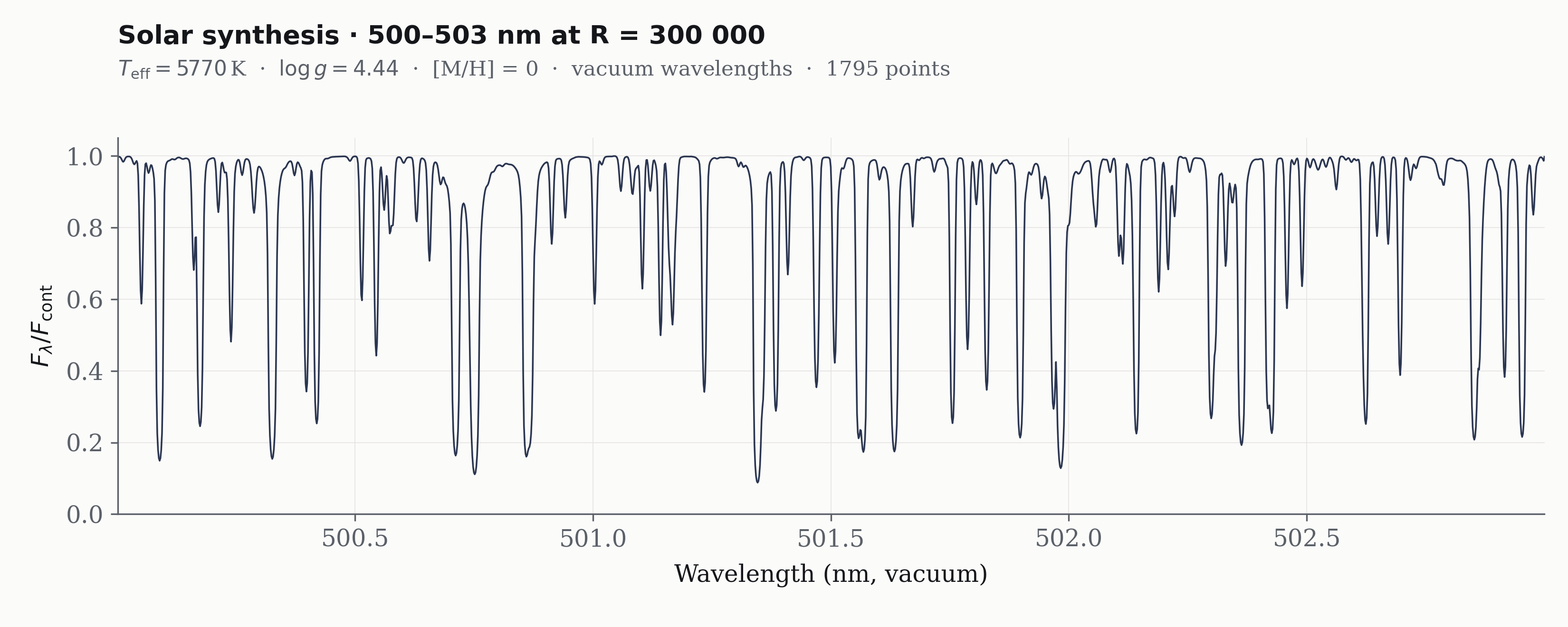
Generated by this pipeline: normalised flux \(F_\lambda / F_{\rm cont}\) for a Sun-like atmosphere (\(T_{\rm eff} = 5770\) K, \(\log g = 4.44\), [M/H] = 0) over a 3 nm chunk at the default \(R = 300\,000\). Dozens of resolved Fe, Ti, Cr, Ni lines populate this dense optical region; their cores reach \(\sim 10\%\) of the continuum and the Voigt wings are clearly visible.
The spectrum is a whitespace-delimited text file with three columns:
| Column | Name | Units | Description |
|---|---|---|---|
| 1 | Wavelength | nm (vacuum) | Wavelength of each sample point |
| 2 | \(F_\lambda\) | erg cm⁻² s⁻¹ nm⁻¹ | Total emergent flux (line + continuum) |
| 3 | \(F_{\rm cont}\) | erg cm⁻² s⁻¹ nm⁻¹ | Continuum-only flux |
The normalized spectrum is simply \(F_\lambda / F_{\rm cont}\). You can read and plot it in Python:
import numpy as np
import matplotlib.pyplot as plt

wl, flux, cont = np.loadtxt(
    "results/spec/t05770g4.44_mh+0.00_am+0.00_500_510.spec",
    unpack=True
)

plt.figure(figsize=(10, 4))
plt.plot(wl, flux / cont, lw=0.5, c="C0")
plt.xlabel("Wavelength (nm)")
plt.ylabel(r"$F_\lambda / F_{\rm cont}$")
plt.title("Solar Spectrum (500–510 nm)")
plt.ylim(0, 1.1)
plt.tight_layout()
plt.savefig("solar_500_510.png", dpi=200)
Why vacuum wavelengths?
pykurucz uses vacuum wavelengths internally because the radiative transfer and line-opacity calculations are most naturally expressed in vacuum. The conversion to air is a simple multiplicative factor if you need to compare against observed spectra tabulated in air.
The .atm file
The iterated atmosphere (t05770g4.44_mh+0.00_am+0.00.atm) is a Kurucz-format text file. It contains:
- Header cards:
TEFF,GRAVITY,TITLE,OPACITY,CONVECTION,ABUNDANCE - Abundance table for elements 1–99
READ DECK6block with 80 layers of atmospheric structure
You can inspect it with any text editor, or load it programmatically:
from atlas_py.io.atmosphere import load_atm

atm = load_atm("results/atm/t05770g4.44_mh+0.00_am+0.00.atm")
print(atm.temperature)   # shape (80,)
print(atm.gas_pressure)  # shape (80,)
The .npz file
The .npz cache contains precomputed quantities that accelerate synthesis:
- Saha–Boltzmann populations for all ions
- Molecular equilibrium partial pressures
- Continuous opacity coefficients
- Doppler widths
It is generated by convert_atm_to_npz.py and consumed by synthe_py.cli. You generally do not need to interact with it directly, but you can load it with numpy.load if you wish to inspect the internal arrays.
Step 4 — Experiment
Two axes to play with: the stellar parameters (\(T_{\rm eff}\), \(\log g\)) and the abundance specification. The atmosphere is rebuilt from scratch each time, so changes to either propagate through to the emergent spectrum self-consistently.
Stellar parameters
# A cool K dwarf
python pykurucz.py --teff 4000 --logg 4.5 --wl-start 650 --wl-end 660

# A hot A star
python pykurucz.py --teff 8250 --logg 4.0 --wl-start 400 --wl-end 410
Bulk abundance changes (--mh, --am)
# Metal-poor α-enhanced K giant — the standard halo / thick-disk knob set
python pykurucz.py --teff 4500 --logg 2.0 --mh -1.5 --am 0.3 \
    --wl-start 500 --wl-end 510
Per-element abundance changes (--abund)
The whole point of driving ATLAS12 (rather than re-using a scaled-solar atmosphere grid) is being able to do this and have the atmosphere respond — not just the line strengths.
# CEMP-s star: Fe-poor, C and Ba enhanced
python pykurucz.py --teff 4800 --logg 1.5 \
    --abund Fe:-2.5 --abund C:+1.2 --abund Ba:+1.0 \
    --wl-start 400 --wl-end 700

# Same metal-poor giant as above but with carbon individually bumped
python pykurucz.py --teff 4500 --logg 2.0 --mh -1.5 --am 0.3 \
    --abund C:+0.6 \
    --wl-start 430 --wl-end 432   # zoom on the CH G-band
Start narrow
For quick experimentation, restrict the wavelength range to 10 nm. Full 300–1800 nm synthesis is much slower but covers the complete optical + NIR.
Next Steps
- Read the User Guide to understand Existing Atmosphere vs. Stellar Parameters in depth.
- Learn about custom abundances and resolution choices.
- Dive into the Physics reference for the details of opacity and radiative transfer.